Histograms - Statistics of Column
 A histogram is a type of Column statistics that provides more detailed information about the data distribution in a table column.
 A histogram sorts values into "buckets".
Below terms and definition used in Doc
NDV - Number of distinct values in a column.
Data Skew – Distribution of Distinct value in column with huge variations. Like for Gender Y value is 80 rows and for Gender X value is 20 rows out of 100 rows. So this is skewed data.
Cardinality - The number of rows that is expected to be or is returned by an operation in an execution plan.
Why Histogram Coined in Oracle
By default the optimizer assumes a uniform distribution of rows across the distinct values in a column.
For columns that contain data skew (a nonuniform distribution of data within the column), a histogram enables the optimizer to generate accurate cardinality estimates for filter and join predicates that involve these columns.
Example => A table column contains 3 NDV as M,F,N and there are 9500 rows for M , 400 rows for F and 100 rows for N .When user queries for N values optimizer will estimate this as uniform distribution ,when there is no Histograms, resulting 10000/3 = 3333 rows and results to FULL tables scan. Whereas if Histogram is there will be index used.
When Oracle Database Creates Histograms
If DBMS_STATS gathers statistics for a table, and if queries have referenced the columns in this table, then Oracle Database creates histograms automatically as needed according to the previous query workload.
The basic process is as follows:
You run DBMS_STATS for a table with the METHOD_OPT parameter set to the default SIZE AUTO.
A user queries the table.
The database notes the predicates in the preceding query and updates the data dictionary table SYS.COL_USAGE$.
You run DBMS_STATS again, causing DBMS_STATS to query SYS.COL_USAGE$ to determine which columns require histograms based on the previous query workload.
Consequences of the AUTO feature include the following:
As queries change over time, DBMS_STATS may change which statistics it gathers. For example, even if the data in a table does not change, queries and DBMS_STATS operations can cause the plans for queries that reference these tables to change.
If you gather statistics for a table and do not query the table, then the database does not create histograms for columns in this table. For the database to create the histograms automatically, you must run one or more queries to populate the column usage information in SYS.COL_USAGE$.
Types of Histograms
1. Frequency
2. Hight-Balanced
3. Hybrid Histogram
4. Top n Frequency
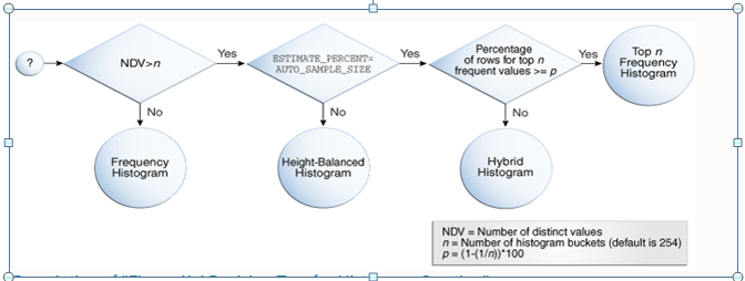
How Oracle Database Chooses the Histogram Type
The histogram formula uses the following variables:
Decision Tree for Histogram Creation
Cardinality Algorithms When Using Histograms
For histograms, the algorithm for cardinality depends on factors such as the endpoint numbers and values, and whether column values are popular or nonpopular.
1 => Endpoint Numbers and Values
An endpoint number is a number that uniquely identifies a bucket. In frequency and hybrid histograms, the endpoint number is the cumulative frequency of all values included in the current and previous buckets.
For example, a bucket with endpoint number 100 means the total frequency of values in the current and all previous buckets is 100. In height-balanced histograms, the optimizer numbers buckets sequentially, starting at 0 or 1. In all cases, the endpoint number is the bucket number.
An endpoint value is the highest value in the range of values in a bucket. For example, if a bucket contains only the values 52794 and 52795, then the endpoint value is 52795.
2 => Popular and Nonpopular Values
The popularity of a value in a histogram affects the cardinality estimate algorithm.
Specifically, the cardinality estimate is affected as follows:
Popular values
A popular value occurs as an endpoint value of multiple buckets. The optimizer determines whether a value is popular by first checking whether it is the endpoint value for a bucket. If so, then for frequency histograms, the optimizer subtracts the endpoint number of the previous bucket from the endpoint number of the current bucket. Hybrid histograms already store this information for each endpoint individually. If this value is greater than 1, then the value is popular.
The optimizer calculates its cardinality estimate for popular values using the following formula
cardinality of popular value = (num of rows in table) * (num of endpoints spanned by this value / total num of endpoints)
A popular value occurs as an endpoint value of multiple buckets. The optimizer determines whether a value is popular by first checking whether it is the endpoint value for a bucket. If so, then for frequency histograms, the optimizer subtracts the endpoint number of the previous bucket from the endpoint number of the current bucket. Hybrid histograms already store this information for each endpoint individually. If this value is greater than 1, then the value is popular.
The optimizer calculates its cardinality estimate for popular values using the following formula
Nonpopular values
Any value that is not popular is a nonpopular value. The optimizer calculates the cardinality estimates for nonpopular values using the following formula:
cardinality of nonpopular value = (num of rows in table) * density
The optimizer calculates density using an internal algorithm based on factors such as the number of buckets and the NDV. Density is expressed as a decimal number between 0 and 1. Values close to 1 indicate that the optimizer expects many rows to be returned by a query referencing this column in its predicate list. Values close to 0 indicate that the optimizer expects few rows to be returned.
3 => Bucket Compression
In some cases, to reduce the total number of buckets, the optimizer compresses multiple buckets into a single bucket.
For example, the following frequency histogram indicates that the first bucket number is 1 and the last bucket number is 23:
Several buckets are "missing." Originally, buckets 2 through 6 each contained a single instance of value 52793. The optimizer compressed all of these buckets into the bucket with the highest endpoint number (bucket 6), which now contains 5 instances of value 52793. This value is popular because the difference between the endpoint number of the current bucket (6) and the previous bucket (1) is 5. Thus, before compression the value 52793 was the endpoint for 5 buckets.
The following annotations show which buckets are compressed, and which values are popular:
| ENDPOINT_NUMBER | ENDPOINT_VALUE |
| 1 | 52792 |
| 6 | 52793 |
| 8 | 52794 |
| 9 | 52795 |
| 10 | 52796 |
| 12 | 52797 |
| 14 | 52798 |
| 23 | 52799 |
| ENDPOINT_NUMBER | ENDPOINT_VALUE | Comments |
| 1 | 52792 | -> nonpopular |
| 6 | 52793 | -> buckets 2-6 compressed into 6; popular |
| 8 | 52794 | -> buckets 7-8 compressed into 8; popular |
| 9 | 52795 | -> nonpopular |
| 10 | 52796 | -> nonpopular |
| 12 | 52797 | -> buckets 11-12 compressed into 12; popular |
| 14 | 52798 | -> buckets 13-14 compressed into 14; popular |
| 23 | 52799 | -> buckets 15-23 compressed into 23; popular |
TYPE OF HISTOGRAM
1=> Frequency Histograms
In a frequency histogram, each distinct column value corresponds to a single bucket of the histogram. Because each value has its own dedicated bucket, some buckets may have many values, whereas others have few.
An analogy to a frequency histogram is sorting coins so that each individual coin initially gets its own bucket. For example, all the Rupees 1 coins are in bucket 1, all the Rupees 2 coins are in bucket 2, all the Rupees 5 coins in bucket 3.
Criteria for Frequency Histograms
The database creates a frequency histogram when the following criteria are met:
NDV is less than or equal to n, where n is the number of histogram buckets (default 254).
The estimate_percent parameter in the DBMS_STATS statistics gathering procedure is set to either a user-specified value or to AUTO_SAMPLE_SIZE.
Starting in Oracle Database 12c, if the sampling size is the default of AUTO_SAMPLE_SIZE, then the database creates frequency histograms from a full table scan. For all other sampling percentage specifications, the database derives frequency histograms from a sample.
Test Case for Frequency Histogram
For below example GENDER column has data skew .As shown below.

SQL> SELECT GENDER,COUNT(*) FROM EMP_DETAILS GROUP BY GENDER;

GENDER   COUNT(*)
---------- ----------
M          900
F          300
N          100

SQL>

SQL> SELECT COUNT(*) FROM EMP_DETAILS;

  COUNT(*)
----------
      1300

Let we create Index on that column as below

SQL> SELECT INDEX_NAME FROM USER_INDEXES WHERE TABLE_NAME='EMP_DETAILS';

no rows selected

SQL> CREATE INDEX EMP_DETAILS_IDX ON EMP_DETAILS(GENDER);

Index created.

SQL> SELECT INDEX_NAME FROM USER_INDEXES WHERE TABLE_NAME='EMP_DETAILS';

INDEX_NAME
--------------------------------------------------------------------------------------------------------------------------------
EMP_DETAILS_IDX

SQL> SELECT TABLE_NAME,COLUMN_NAME,NUM_DISTINCT,HISTOGRAM FROM USER_tAB_COL_STATISTICS WHERE TABLE_NAME='EMP_DETAILS';

TABLE_NAME         COLUMN_NAME      NUM_DISTINCT HISTOGRAM
-------------------- -------------------- ------------ ---------------
EMP_DETAILS         ID                     1300 NONE
EMP_DETAILS         GENDER                 3    NONE

Let we gather stats with DBMS_STATS.AUTO_SAMPLE_SIZE

SQL> exec dbms_stats.gather_table_stats(ownname=>'abhi_test',tabname=>'EMP_DETAILS',estimate_percent=>DBMS_STATS.AUTO_SAMPLE_SIZE,cascade=>TRUE,degree =>4);

PL/SQL procedure successfully completed.

Before Histogram

Let we check Cardinality estimate for GENDER='N'

SQL> EXPLAIN PLAN FOR SELECT * FROM EMP_DETAILS WHERE GENDER='N';

Explained.

SQL>
SQL> SELECT * FROM DBMS_XPLAN.DISPLAY();

PLAN_TABLE_OUTPUT
----------------------------
Plan hash value: 1421366555

-------------------------------------------------------------------------------------------------------
| Id  | Operation			    | Name	      | Rows  | Bytes | Cost (%CPU)| Time     |
-------------------------------------------------------------------------------------------------------
|   0 | SELECT STATEMENT		    |		      |   433 |  2598 |     3	(0)| 00:00:01 |
|   1 |  TABLE ACCESS BY INDEX ROWID BATCHED| EMP_DETAILS     |   433 |  2598 |     3	(0)| 00:00:01 |
|*  2 |   INDEX RANGE SCAN		    | EMP_DETAILS_IDX |   433 |       |     1	(0)| 00:00:01 |
-------------------------------------------------------------------------------------------------------

Predicate Information (identified by operation id):

PLAN_TABLE_OUTPUT
--------------------------------------------------

   2 - access("GENDER"='N')

14 rows selected.

SQL> SELECT TABLE_NAME,COLUMN_NAME,HISTOGRAM FROM USER_tAB_COL_STATISTICS WHERE TABLE_NAME='EMP_DETAILS';

TABLE_NAME	     COLUMN_NAME	  HISTOGRAM
-------------------- -------------------- ---------------
EMP_DETAILS	     ID 		  NONE
EMP_DETAILS	     GENDER		  NONE

Let we again execute stats gather and see if HISTOGRAMS developed

SQL> exec dbms_stats.gather_table_stats(ownname=>'abhi_test',tabname=>'EMP_DETAILS',estimate_percent=>DBMS_STATS.AUTO_SAMPLE_SIZE,cascade=>TRUE,degree =>4);

PL/SQL procedure successfully completed.

Post Histogram

SQL>
SQL>
SQL>
SQL> SELECT TABLE_NAME,COLUMN_NAME,HISTOGRAM FROM USER_tAB_COL_STATISTICS WHERE TABLE_NAME='EMP_DETAILS';

TABLE_NAME      COLUMN_NAME   HISTOGRAM
-------------------- -------------------- ---------------
EMP_DETAILS      ID         NONE
EMP_DETAILS      GENDER    FREQUENCY

SQL>

Now let we again Explain above query again and check Cardinality Estimate as below,

SQL> SELECT TABLE_NAME,COLUMN_NAME,HISTOGRAM FROM USER_tAB_COL_STATISTICS WHERE TABLE_NAME='EMP_DETAILS';

TABLE_NAME	     COLUMN_NAME	  HISTOGRAM
-------------------- -------------------- ---------------
EMP_DETAILS	     ID 		  NONE
EMP_DETAILS	     GENDER		  FREQUENCY

SQL>
SQL>
SQL>  EXPLAIN PLAN FOR SELECT * FROM EMP_DETAILS WHERE GENDER='N';

Explained.

SQL>
SQL>
SQL>  SELECT * FROM DBMS_XPLAN.DISPLAY();

PLAN_TABLE_OUTPUT
---------------------------------------------
Plan hash value: 1421366555

-------------------------------------------------------------------------------------------------------
| Id  | Operation			    | Name	      | Rows  | Bytes | Cost (%CPU)| Time     |
-------------------------------------------------------------------------------------------------------
|   0 | SELECT STATEMENT		    |		      |   100 |   600 |     2	(0)| 00:00:01 |
|   1 |  TABLE ACCESS BY INDEX ROWID BATCHED| EMP_DETAILS     |   100 |   600 |     2	(0)| 00:00:01 |
|*  2 |   INDEX RANGE SCAN		    | EMP_DETAILS_IDX |   100 |       |     1	(0)| 00:00:01 |
-------------------------------------------------------------------------------------------------------

Predicate Information (identified by operation id):

PLAN_TABLE_OUTPUT
--------------------------------------------------

   2 - access("GENDER"='N')

14 rows selected.

SQL> SELECT TABLE_NAME,COLUMN_NAME,NUM_DISTINCT,HISTOGRAM FROM USER_TAB_COL_STATISTICS WHERE TABLE_NAME='EMP_DETAILS';

TABLE_NAME	     COLUMN_NAME	  NUM_DISTINCT HISTOGRAM
-------------------- -------------------- ------------ ---------------
EMP_DETAILS	     ID 			  1300 NONE
EMP_DETAILS	     GENDER			     3 FREQUENCY

SQL> SELECT COUNT(*) FROM EMP_DETAILS;

  COUNT(*)
----------
      1300

SQL> SELECT GENDER,COUNT(*) FROM EMP_DETAILS GROUP BY GENDER;

G   COUNT(*)
- ----------
M	 900
F	 300
N	 100
SQL>
SQL>  SELECT TABLE_NAME,COLUMN_NAME,ENDPOINT_NUMBER FROM USER_HISTOGRAMS WHERE TABLE_NAME='EMP_DETAILS' AND COLUMN_NAME='GENDER';

TABLE_NAME	     COLUMN_NAME	  ENDPOINT_NUMBER
-------------------- -------------------- ---------------
EMP_DETAILS	     GENDER			      300
EMP_DETAILS	     GENDER			     1200
EMP_DETAILS	     GENDER			     1300

SQL>


So as we can see after HISTOGRAM build up Cardinality estimation got corrected as GENDER='N' are ~ 100 rows in table.

Generating a Frequency Histogram

To generate FREQUENCY HISTOGRAM below condition has to met.

1-> Data Skew in Column.
2-> NDV < n where as n=254 (default)
3-> DBMS_STATS must be used with auto_sampling as below,
exec dbms_stats.gather_table_stats(ownname=>'abhi_test',tabname=>'EMP_DATA',estimate_percent=>DBMS_STATS.AUTO_SAMPLE_SIZE,cascade=>TRUE,degree =>4);|

So after running query multiple times HISTOGRAM got created, once above criteria met.
2=> Top-n Frequency Histograms
A top frequency histogram is a variation on a frequency histogram that ignores nonpopular values that are statistically insignificant.
For example, if a pile of 1000 coins contains only a coin of 1 rupees then you can ignore the only 1 coin when sorting the coins into buckets. A top frequency histogram can produce a better histogram for highly popular values.
Criteria for Top Frequency Histograms
If a small number of values occupies most of the rows, then creating a frequency histogram on this small set of values is useful even when the NDV is greater than the number of requested histogram buckets. To create a better quality histogram for popular values, the optimizer ignores the nonpopular values and creates a top frequency histogram.
The database creates a TOP frequency histogram when the following criteria are met:
NDV is greater than n, where n is the number of histogram buckets (default 254).
The percentage of rows occupied by the top threshold p, where p is (1-(1/n))*100.
The estimate_percent parameter in the DBMS_STATS statistics gathering procedure is set to AUTO_SAMPLE_SIZE.
Data Skew
Test Case for Top-n Frequency Histogram
Here to demonstrate we need to shorten BUCKET Size i.e “n” .For that DBMS_STATS provide below method.

method_opt => 'FOR COLUMNS '

SQL> SELECT GENDER,COUNT(*) FROM EMP_TEST_TOPN GROUP BY GENDER;

GENDER	     COUNT(*)
---------- ----------
M		  500
F		  100
N		  400
S		  100
V		  500
T		  400

6 rows selected.

SQL>
SQL>
SQL> SELECT TABLE_NAME,COLUMN_NAME,NUM_DISTINCT,HISTOGRAM FROM USER_TAB_COL_STATISTICS WHERE TABLE_NAME='EMP_TEST_TOPN';

TABLE_NAME	     COLUMN_NAME	  NUM_DISTINCT HISTOGRAM
-------------------- -------------------- ------------ ---------------
EMP_TEST_TOPN	     ID 			  2000 NONE
EMP_TEST_TOPN	     GENDER			     6 NONE

SQL>
SQL>
SQL> EXPLAIN PLAN FOR SELECT * FROM EMP_TEST_TOPN WHERE GENDER='S';

Explained.

SQL> SELECT * FROM DBMS_XPLAN.DISPLAY();

PLAN_TABLE_OUTPUT
-----------------------------------------------------------------------------------
Plan hash value: 2365112915

-----------------------------------------------------------------------------------
| Id  | Operation	  | Name	  | Rows  | Bytes | Cost (%CPU)| Time	  |
-----------------------------------------------------------------------------------
|   0 | SELECT STATEMENT  |		  |   333 |  1998 |	4   (0)| 00:00:01 |
|*  1 |  TABLE ACCESS FULL| EMP_TEST_TOPN |   333 |  1998 |	4   (0)| 00:00:01 |
-----------------------------------------------------------------------------------

Predicate Information (identified by operation id):
---------------------------------------------------

PLAN_TABLE_OUTPUT
----------------------------
   1 - filter("GENDER"='S')

13 rows selected.

SQL>
SQL>

Here NDV =6 so we need to have n as less than 6 ,To achieve this we use below porc.

SQL> exec dbms_stats.gather_table_stats(ownname=>'abhi_test',tabname=>'EMP_TEST',estimate_percent=>DBMS_STATS.AUTO_SAMPLE_SIZE,method_opt => 'FOR COLUMNS GENDER SIZE 5',cascade=>TRUE;

PL/SQL procedure successfully completed.
SQL>
SQL> SELECT TABLE_NAME,COLUMN_NAME,NUM_DISTINCT,HISTOGRAM FROM USER_TAB_COL_STATISTICS WHERE TABLE_NAME='EMP_TEST_TOPN';

TABLE_NAME	     COLUMN_NAME	  NUM_DISTINCT HISTOGRAM
-------------------- -------------------- ------------ ---------------
EMP_TEST_TOPN	     ID 			  2000 NONE
EMP_TEST_TOPN	     GENDER			     6 TOP-FREQUENCY

SQL>
SQL> EXPLAIN PLAN FOR SELECT * FROM EMP_TEST_TOPN WHERE GENDER='S';

Explained.

SQL>  SELECT * FROM DBMS_XPLAN.DISPLAY();

PLAN_TABLE_OUTPUT
---------------------------------------
Plan hash value: 2365112915

-----------------------------------------------------------------------------------
| Id  | Operation	  | Name	  | Rows  | Bytes | Cost (%CPU)| Time	  |
-----------------------------------------------------------------------------------
|   0 | SELECT STATEMENT  |		  |   199 |  1194 |	4   (0)| 00:00:01 |
|*  1 |  TABLE ACCESS FULL| EMP_TEST_TOPN |   199 |  1194 |	4   (0)| 00:00:01 |
-----------------------------------------------------------------------------------

Predicate Information (identified by operation id):
---------------------------------------------------

PLAN_TABLE_OUTPUT
--------------------------------------------

   1 - filter("GENDER"='S')

13 rows selected.

Let we check Number of Buckets formed for this Table Columns as below .

SQL>
SQL> SELECT TABLE_NAME,COLUMN_NAME,ENDPOINT_NUMBER FROM USER_HISTOGRAMS WHERE TABLE_NAME='EMP_TEST_TOPN'  AND COLUMN_NAME='GENDER';

TABLE_NAME	     COLUMN_NAME	  ENDPOINT_NUMBER
-------------------- -------------------- ---------------
EMP_TEST_TOPN	     GENDER				  1
EMP_TEST_TOPN	     GENDER			      501
EMP_TEST_TOPN	     GENDER			      901
EMP_TEST_TOPN	     GENDER			     1301
EMP_TEST_TOPN	     GENDER			     1801

As we can see there are 5 bucket avialble for GENDER colmn due to Method_opt value in DBMS_STATS.

SQL>
SQL> SELECT GENDER,COUNT(*) FROM EMP_TEST_TOPN GROUP BY GENDER;

GENDER	     COUNT(*)
---------- ----------
M		  500
F		  100
N		  400
S		  100
V		  500
T		  400

6 rows selected.

Now let we verify requirement for TOP-Frequency .

1=> NDV > n  i.e  6>5

2=> Value of p

1/5=.2 => 1-.02 => .8 *100 => 80 %
P= 80%

The percentage of rows occupied by the top 5 frequent values is equal to or greater than threshold p,  90% > 80%.
3=> Height-Balanced Histograms (Legacy)
In a legacy height-balanced histogram, column values are divided into buckets so that each bucket contains approximately the same number of rows.

For example, if you have 99 coins to distribute among 4 buckets, each bucket contains about 25 coins. The histogram shows where the endpoints fall in the range of values.

Criteria for Height-Balanced Histograms

The database creates a height-balanced histogram when the following criteria are met:

NDV is greater than n, where n is the number of histogram buckets (default 254).
The estimate_percent parameter in the DBMS_STATS statistics gathering procedure is not set to AUTO_SAMPLE_SIZE.

Generating a Height-Balanced Histogram

Here to demonstrate we need to shorten BUCKET Size i.e “n” .For that DBMS_STATS provide below method. And we also need to set estimate_percent as per user value.
We are continuing with last expample as covered above.

SQL> exec dbms_stats.gather_table_stats(ownname=>'abhi_test',tabname=>'EMP_TEST_TOPN',estimate_percent=>90,method_opt => 'FOR COLUMNS GENDER SIZE 5',cascade=>TRUE,degree =>4);

PL/SQL procedure successfully completed.

SQL> SQL>
SQL> SELECT TABLE_NAME,COLUMN_NAME,NUM_DISTINCT,HISTOGRAM FROM USER_TAB_COL_STATISTICS WHERE TABLE_NAME='EMP_TEST_TOPN';

TABLE_NAME	     COLUMN_NAME	  NUM_DISTINCT HISTOGRAM
-------------------- -------------------- ------------ ---------------
EMP_TEST_TOPN	     ID 			  2000 NONE
EMP_TEST_TOPN	     GENDER			     6 HEIGHT BALANCED

SQL>
4=> Hybrid Histograms
A hybrid histogram combines characteristics of both height-based histograms and frequency histograms. This "best of both worlds" approach enables the optimizer to obtain better selectivity estimates in some situations.
The height-based histogram sometimes produces inaccurate estimates for values that are almost popular. For example, a value that occurs as an endpoint value of only one bucket but almost occupies two buckets is not considered popular.
To solve this problem, a hybrid histogram distributes values so that no value occupies more than one bucket, and then stores the endpoint repeat count value, which is the number of times the endpoint value is repeated, for each endpoint (bucket) in the histogram. By using the repeat count, the optimizer can obtain accurate estimates for almost popular values.
Criteria for Hybrid Histograms
The database creates a hybrid histogram when the following criteria are met:

NDV is greater than n, where n is the number of histogram buckets (default is 254).
The percentage of rows occupied by the top n frequent values is less than threshold p, where p is (1-(1/n))*100.
The estimate_percent parameter in the DBMS_STATS statistics gathering procedure is set to AUTO_SAMPLE_SIZE.
Generating a Height-Balanced Histogram
Here to demonstrate we need to shorten BUCKET Size i.e “n” .For that DBMS_STATS provide below method. And we also need to set estimate_percent as per DBMS_STATS.AUTO_SAMPLE_SIZE.
We are continuing with last expample as covered above.
SQL>
SQL> exec dbms_stats.gather_table_stats(ownname=>'abhi_test',tabname=>'EMP_TEST_TOPN',estimate_percent=>DBMS_STATS.AUTO_SAMPLE_SIZE,method_opt => 'FOR COLUMNS GENDER SIZE 2',cascade=>TRUE);

PL/SQL procedure successfully completed.

SQL> SELECT TABLE_NAME,COLUMN_NAME,NUM_DISTINCT,HISTOGRAM FROM USER_TAB_COL_STATISTICS WHERE TABLE_NAME='EMP_TEST_TOPN';

TABLE_NAME      COLUMN_NAME   NUM_DISTINCT HISTOGRAM
-------------------- -------------------- ------------ ---------------
EMP_TEST_TOPN      ID      2000 NONE
EMP_TEST_TOPN      GENDER        6 HYBRID

SQL> SELECT TABLE_NAME,COLUMN_NAME,ENDPOINT_NUMBER,ENDPOINT_REPEAT_COUNT FROM USER_HISTOGRAMS WHERE TABLE_NAME='EMP_TEST_TOPN'  AND COLUMN_NAME='GENDER';

TABLE_NAME         COLUMN_NAME      ENDPOINT_NUMBER ENDPOINT_REPEAT_COUNT
-------------------- -------------------- --------------- ---------------------
EMP_TEST_TOPN         GENDER                  100            100
EMP_TEST_TOPN         GENDER                 2000            500

SQL>
SQL>
Views Used for HISTOGRAMS
USER_TAB_COL_STATISTICS
USER_HISTOGRAMS
USER_TAB_COLUMNS
© 2021 Ace2Oracle. All Rights Reserved | Developed By IBOX444